3D EM boundary element solver

HyperLynx Full-Wave Solver

The HyperLynx Full Wave Solver (FWS) is a boundary element solver used for simulating the very-high frequency behavior of 3D electromagnetic structures that have arbitrary geometries. It is one member of the integrated family of HyperLynx Advanced Solvers.

Full-wave solver applications

Full-wave approaches are used when the structure being analyzed is comparable (or larger) than the signal wavelength at the frequencies of interest. This is a general-purpose approach that doesn't make assumptions about the structure's geometry or its electromagnetic behavior. In HyperLynx, the full-wave solver is typically used to model critical sections of high-speed serial channels (breakouts, blocking caps, vias & other discontinuities), sections of high-density IC packages or selected portions of DDR5 memory interfaces.

Full-wave solutions provide the most accurate simulations currently available. This also means that they are the most complex and memory intensive, making them the most likely to require simulation acceleration, either by use of many CPU cores on large server, or by splitting the job (or jobs) across multiple machines on a LAN.

HyperLynx integration and ease of use

When full-wave solvers are used as part of system-level analysis, the full interconnect is normally too large to be practically solved with a 3D solver. That means that interconnect gets partitioned into sections that require a 3D solver (breakout regions, vias and blocking caps), sections that can be accurately described with trace models, and sections represented as S-parameter models (often connectors and IC packages). This is known as "cut and stitch" solving - the interconnect is "cut" into sections that are each modeled individually, then the pieces are "stitched" back together to create an end to end channel model for system level analysis.

The cut and stitch method maximizes solving efficiency because the size of the areas solved with 3D simulation are limited to critical signal areas and their respective return paths. Outside those areas, representing the signal with a trace or connector model is far more efficient from a compute time and resource standpoint. The challenge with the cut and stitch method is managing all the details correctly - for example, each 3D area needs to be large enough to ensure Transverse Electro Magnetic (TEM) behavior at the port boundaries. This means that the area will include some portion of the signal trace, and the trace length modeled as a transmission line will need to be adjusted to reflect the portion of trace already included in the 3D area. That 3D area also needs to include the signal's return path, so ground stitching vias and an adequate buffer distance also need to be considered when creating the area. Normally, this process is done by hand, requiring considerable user expertise. This vastly limits the number of users who can perform the analysis, and the number of signals they can practically analyze.

HLAS-integration and ease of use 1280

Automated post-layout channel model creation

HyperLynx automatically creates post-layout channel models based on requirements for the protocol being analyzed. Users simply select the signals they want to analyze, and HyperLynx does the rest:

  • The built-in DRC engine is used to automatically identify sections of the interconnect that require 3D modeling.
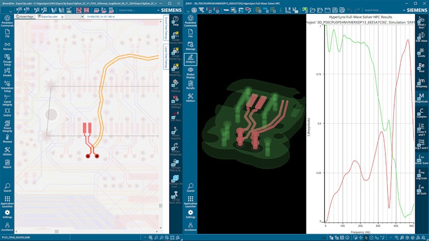
  • HyperLynx BoardSim creates the appropriate setups for 3D simulation and sends them to the full-wave solver.
  • The full-wave solver models the 3D areas to the required frequency and creates models for SI analysis. These models include port metadata that indicates how they should be connected within the full channel model.
  • BoardSim combines the models from the 3D simulator with trace and connector models to create a model that represents the channel.
  • BoardSim then runs protocol-aware SI simulation (typically SerDes or DDR analysis) to establish operating margins at the system level. This tells the user which signals pass, which fail and by how much.

Comprehensive visualization & post processing

HyperLynx's Full-wave Solver includes a full set of output plotting facilities that show behavior and update in real time as a simulation progresses, allowing the user to see how the model is evolving as the simulation is run. These include plots of real, magnitude, imaginary and phase behavior, displayed with linear, log and dB scales. Polar plotting is also supported.

Once the simulation is complete, animated current and field density plots can be used to further investigate the structure's behavior.

Simulated results can be post-processed to de-embed effects of port structures, check for and enforce passivity, split large matrices into smaller ones, adjust port reference termination values and convert single-ended data to mixed-mode data.

Simulation models can be exported as S-,Y- and Z-parameter data with spice wrapper subcircuits for inclusion in system-level circuit simulations. Generated models also include port metadata that defines what each port represents and how it should be connected into a larger model for system-level simulations.

full wave solver reporting

Scalable performance

Full-wave solving is the most compute and memory intensive of all solver applications, because it provides the greatest accuracy and makes the fewest assumptions about the structure being solved. HyperLynx uses a two-tiered strategy for improving solver throughput:

  • The first (and simplest) performance tier involves adding more CPU cores to an individual solver run. In this scenario, the solver distributes tasks among the available cores to get the job completed faster. The user controls how many cores each solver job is allowed to use. Like any distributed analysis process, adding more cores eventually hits a point of diminishing returns. At that point, if the simulation is being run on a large server, several simulations can be run in parallel to increase throughput.
  • The second tier involves distributing multiple solver runs to different machines across a LAN. This allows simulation performance to be scaled to very high levels, particularly when there are a large number of solver jobs to run. HyperLynx Advanced Solvers Job Distribution (HL-AS JD) provides a solver job management layer that allows users to control how and where simulation jobs will be executed. HL-AS JD can distribute and manage simulation jobs across the LAN directly, or it can interface to commercial load management systems (LSF, Windows HPC) to take advantage of existing analysis infrastructure where available.
HLAS - HyperLynx Scalable Peformance 1280x720

Scripting & automation

Signal and Power Integrity Analysis are complex, multi-step processes, where changing a single option can significantly affect the end result. Because these simulations are often lengthy, compute and memory-intensive, ensuring that simulations are set up properly and performed consistently is critical. Without the ability to ensure that simulations are performed consistently and accurately, much time is lost adjusting and resimulating.

HyperLynx Advanced Solvers can be run both interactively and through Python-based automation. This allows designs to be initially set up, analyzed and debugged using interactive analysis to determine optimal simulation settings. Then, as the design is iterated, those settings can be reused through automation to ensure analysis is always run the same way, reports the same metrics and produces the same output models. An interactive, command-line scripting environment is available directly with the solvers so that users can develop and test their automation scripts.

HyperLynx Advanced Solver automation is part of a broader scripting framework for the full HyperLynx family, that allows automated multi-tool analysis flows to be created. This object-oriented scripting framework includes pre-defined flows for power integrity, signal integrity and serial link compliance analysis that allow users to run complex analyses with just a few lines of custom code.

HyperLynx Scripting and Automation
Full-wave solver

Resources