SHERPA exploration algorithm

HyperLynx Design Space Exploration

HyperLynx Design Space Exploration (HL-DSE) provides advanced design optimization when the number of simulation cases to be investigated vastly exceeds what is practical. HL-DSE can find optimal solutions with a fraction of the computational resources required by traditional methods.

The edge of a monitor featuring HyperLynx Design Space Exploration design optimization for large simulations using simple iteration, swept-parameter analysis or surface response modeling analysis.

The optimization challenge

Simulation lets designers analyze, debug and optimize an electronic design using a digital twin before releasing a prototype to fabrication. This results in a more robust, reliable and cost-effective board by reducing the likelihood of issues arising during lab testing which may require a board respin.

Simulation also allows users to explore alternative versions of their design to improve reliability, speed or margin, or to reduce the overall manufacturing cost. When simulation is used as an optimization tool, the complexity of the analysis performed normally increases in stages:

Select...

Initially, users modify the design and re-simulate changes one at a time. This works well for simple studies and is easy for new simulation users to understand. This method works best when there are only one or two design parameters (variables) to be studied and when the user can readily determine the parameter values to use for the next study based on the results of previous ones.

Fast, efficient optimization

Efficiently exploring large design spaces with as few simulations as possible is a difficult task that requires a combination of advanced analysis techniques. This requires an approach that balances two conflicting requirements:

  1. Zeroing in on any promising results to find their optimal values quickly. When a design space is initially sampled, the values picked rarely result in optimum values. Instead, they produce gradients, that are processed to find optimum locations (usually local maxima/minima) on the response surface. Zeroing in on a locally (but not globally) optimal result requires additional simulation experiments that ultimately don't contribute to finding the global optimum.
  2. Ensuring that the entire design space is adequately sampled. Consider an egg carton where the peaks and valleys are all slightly different. There are many different local minima and maxima - but only one global value of each. It's easy to find a local gradient and the local peak/valley after initial sampling - but very difficult to ensure that the global value is found. The entire space must be sampled adequately enough that the global maxima/minima have been found by the end of the process.

SHERPA algorithm

Balancing these two different requirements is a difficult task that requires advanced techniques to assess each response as it becomes available to evaluate the numerical order of the response surface and determine the next experiment to run. With most optimizers, this requires considerable understanding of both the problem being solved and the search algorithm itself to "tune" the control parameters for the algorithm.

With HL-DSE, the SHERPA algorithm evaluates responses as the analysis runs and tunes the algorithm automatically. HL-DSE produces a plot of the responses as the analysis proceeds, showing the value(s) obtained from each simulation experiment.

HyperLynx graph showing a design of experiments optimization history shown via SHERPA algorithm

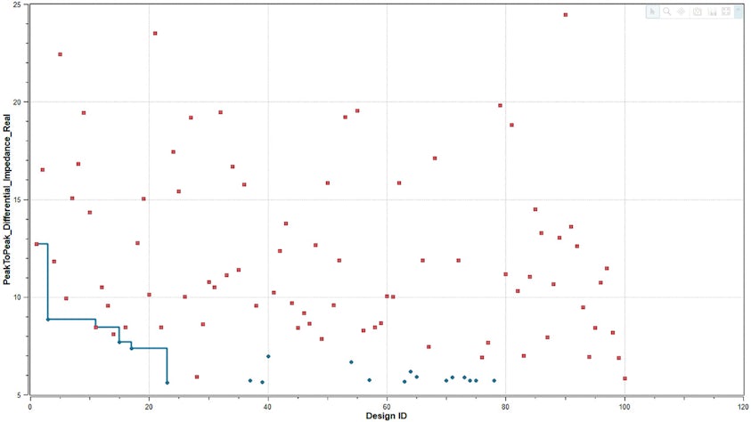
In this plot, HL-DSE has two figures of merit and associated goals:

  • optimize red values
  • minimize blue values

The blue line shows the history of experiments which improved the value of the blue metric. 100 simulations were given as the budget for this analysis, out of a total of 82,500 possible permutations of input values.

Within 25 simulations SHERPA was able to quickly find near optimal values for each metric.

Response Surface Methodology

Results visualization

Due to the complex nature of the problems being investigated, advanced optimization techniques are able to sample only a small percentage of the total design space. Being able to visualize analysis results quickly and effectively is a key part to performing processes like via optimization.

HyperLynx Design Space Exploration offers a rich assortment of output plotting capabilities to provide insight into how the design behaves. These include 3D plots that can show things like how return loss is affected by via separation and antipad diameter.

In this example, return loss is to be maximized to improve signal integrity. This involves post-processing each simulation's results to report the maximum value encountered as the response metric, then finding the input variable conditions that minimize that response.

Graph visualization of HyperLynx Design Space Explorer results visualization for surface response modeling and design of experiments and via optimization

Response surface methodology from HyperLynx DSE

Portion of a screen shot showing HyperLynx Desiign Space Exploration pre-layout serial link compliance design table for performing swept-parameter analysis and automatic PCB optimization

Defining the design space

HL-DSE is integrated with both the HyperLynx Advanced Solvers 3D Explorer and HyperLynx Signal Integrity pre-layout serial link compliance flows, each of which is already capable of performing design optimization through swept-parameter analysis.

When the number of simulation cases becomes untenable, HL-DSE is used to perform automated optimization. Design variables and ranges already defined by the user are communicated to HL-DSE, which the user can review and adjust as necessary.

Analysis Goals

Defining optimization goals

HL-DSE is tightly integrated with 3D Explorer and pre-layout compliance analysis from a simulation output (response) perspective. Output metrics already defined by the user are passed to HL-DSE, where the user adds pass/fail requirements and optimization goals.

individual screen shot showing a portion of the software featuring Design Space Exploration and showing the study responses parameters for impedance and insertion loss.

Surrogate modeling

HyperLynx screen shot showing how surrogate modeling can replace simulation experiment for large models like calculating peak to peak differential impedance. In it is a chart and scatter plot of peak to peak impedance values.

In some applications, simply performing simulation experiments and finding optimal configurations isn't enough, because knowing how the design behaves over millions of cases is the goal. For instance, once a design is optimized, the user may want to predict manufacturing yield over millions of units. In this case, the variables are the design's parameters, but their range becomes the distribution of values one would expect to see as the result of manufacturing tolerances.

Running millions of simulation experiments is clearly not practical, so a fitted mathematical, or surrogate, model is created that closely matches the designs input/output behavior within the parameter range. This surrogate model can then be in used in place of actual simulation experiments to predict the design's behavior over a large number of conditions, and therefore predict manufacturing yield.

Resources